Signal detection theory is a theoretical framework for understanding how decisions are made under uncertainty. It applies whenever judgments must be based on noisy, imperfect evidence—such as deciding whether a faint stimulus was present, whether a face was seen before, whether a medical test result indicates disease, or whether a defendant is guilty. In such situations, observed accuracy reflects not only how well evidence from two states of the world can be distinguished (discriminability) but also how decisively or cautiously the decision maker sets their criterion for responding (response bias). Signal detection theory (SDT) provides principled measures that separate these two components, allowing performance to be conceptualized and quantified in a theoretically coherent way. Although the core ideas underlying SDT date back more than a century, they remain essential today because intuition and simple accuracy measures based on alternative theories often confound sensitivity and bias, leading researchers to draw misleading conclusions. This article reviews the central concepts of SDT, explains the computation and interpretation of its key measures, and considers its enduring foundational role across psychology, neuroscience, medicine, and related fields.
History
The historical roots of SDT lie in an insight that was foundational for experimental psychology: subjective experience can be treated as a noisy measurement. In his work on psychophysics, Gustav Fechner (1860/1966) proposed that when a person perceives a stimulus—such as the heaviness of a weight—the resulting sensation varies from trial to trial because of random noise in the nervous system. As a result, judgments are sometimes incorrect, and not because the observer is guessing but because the internal signal itself fluctuates. This way of thinking transformed errors from nuisances into informative data because the pattern of errors reveals how strongly two stimuli can be discriminated. SDT ultimately grew out of this realization, which provided a principled framework for measuring psychological sensitivity in the presence of unavoidable noise.
Fechner’s proposal was motivated by earlier work on measurement error in the physical sciences. In the early 1800s, the mathematician Carl Friedrich Gauss showed that repeated measurements of the same physical quantity tend to vary around a true value in a systematic way, forming what is now called the normal (or Gaussian) distribution, illustrated schematically in Figure 1A. The key insight was that variability is not merely random chaos but follows lawful statistical regularities that can be characterized by a mean and a dispersion. Although Gauss developed these ideas to understand error in physical measurement, they provided a natural model for thinking about variability in psychological measurements as well, from which internal signals cannot be observed directly. This statistical perspective made it possible to quantify differences between underlying signals in standardized units, laying the groundwork for later developments in psychophysics and, eventually, SDT.
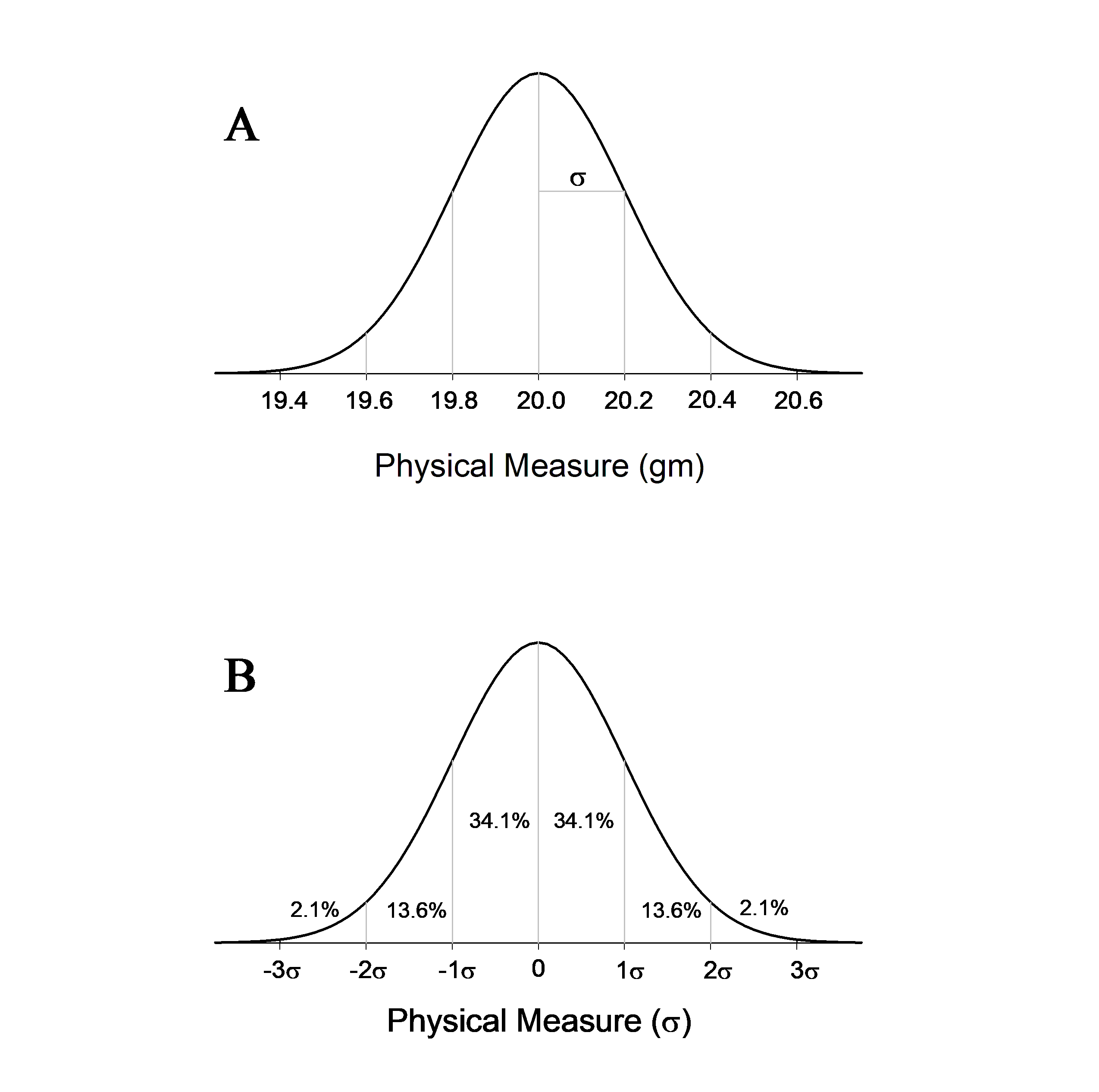
(A) Hypothetical Gaussian distribution of measurements when weighing a 20-gm mass on a balance scale. The mean of many measurements (µ) will be 20 gm, and the hypothetical standard deviation (σ) associated with using this noisy measurement method is 0.2 gm. (B) The same distribution of physical measurements but with the units converted to σ (so that each value is expressed as the number of standard deviations it lies from the mean), a universal metric that applies to all Gaussian distributions.
Figure 1B illustrates the Gaussian distribution with the metric (gm in this case) replaced by
Fechner’s insight about noisy psychological measurement can be illustrated with a simple example involving the perception of weight. When you pick up a small weight, you immediately experience how heavy it feels. In a way, your brain just “measured” the heaviness of that weight. Even though we cannot see this measurement, it exists, and it has some magnitude. We might represent this unobservable quantity as
Imagine that you pick up two small weights, one in each hand, that differ slightly in mass (e.g., weight A = 20 gm and weight B = 18 gm). The heavier weight A in your left hand might feel slightly heavier than weight B in your right hand. If you now repeat that comparison a number of times, you may discover that, occasionally, weight B feels heavier than weight A. The fact that you make an occasional error might seem utterly mundane. However, like Pavlov watching his dog salivate, Fechner thought about Gaussian measurement error and realized that something interesting was happening. Sometimes, random measurement error in the brain may be why the subjective heaviness of the two weights differ from their objective weights. And if the errors are large enough on a given trial, the weight in your right hand (the lighter weight) may subjectively feel heavier than the weight in your left hand. A subtle but important point is that, from the perspective of SDT, errors do not reflect random guesses. Instead, they reflect actual subjective perceptions that differ from objective reality because of random “noise” in the nervous system.
The feelings of heaviness generated by weight A can be conceptualized as a Gaussian distribution with mean
Many years later, Louis Thurstone (1927) realized that this same approach could be used to scale the psychological distance between attributes that cannot even be measured in the observable world. For example, when presented with a choice between Brand A and Brand B, the proportion of a population expressing a preference for Brand B could be used to psychologically scale the magnitude of the difference between the two brands. A few decades later, experimental psychologists and statisticians realized that the psychological distance between two categories could be measured even if only one option was presented at a time—a yes/no task (Tanner & Swets, 1954)—rather than presenting both options simultaneously for a choice—a two-alternative forced-choice task. A real-world example is the criminal trial, in which the decision involves two underlying states of the world—guilty or innocent—but, unlike a forced-choice task, only a single option (the defendant, who is either innocent or guilty) is presented at a given time, and the decision is based on noisy and imperfect evidence (e.g., does the evidence indicate that the defendant is guilty, yes or no?). Many other examples of yes/no detection tasks can be found in the field of psychological science (e.g., did this word appear on an earlier list? Was a quiet tone played on this trial? Is this fake news?).
Core concepts
When using a simple yes/no signal detection task, it is important to conceptualize the data through the lens of SDT. Otherwise, a researcher will probably rely on an intuitive but theoretically incoherent measure to compute an accuracy score for each participant. And if the performance measure is theoretically incoherent, the ability to acquire a deeper theoretical understanding of the question addressed by the research will be on the wrong path from the start.
Every measure of accuracy implies a theory, and it is hard to overstate the importance of that point (Swets, 1986). Even a measure as seemingly straightforward as “percent correct” implies a theory about how the participant is using underlying (unobservable) signals to make a decision. The easiest way to appreciate this point is to consider a concrete example of a signal detection task in which different measures disagree about what the results imply.
Response bias
Consider a recognition memory task in which each participant studies a list of 25 faces randomly selected from a face database and later completes a recognition memory test [see Face Perception]. On this test, suppose that the participant is presented with those same 25 faces again, one at a time, and asked, “Was this one of the faces you saw earlier, yes or no?” If the participant says “Yes” to all 25 faces (100% correct), it might seem to reflect good memory for the studied faces. However, the truth is that you cannot tell if the participant’s memory for these faces is good or bad. The participant may have recognized all 25 faces as having been seen before (good memory), or the participant might be a complete amnesic who does not remember any of the faces but who tends to say “yes” to every presented face anyway (bad memory). In the latter case, we would say that the participant has a strong response bias to say “yes.” Response bias is an issue that must somehow be factored out of the performance score so as not to distort our assessment of a participant’s memory-based performance [see Computational Models of Memory].
This example illustrates how easy it can be to overlook the fact that this recognition task is a signal detection task, with two states of the world (old items that appeared on the list and new items that did not). Critically, in a signal detection task, items from both states must be tested to assess performance. To this day, presenting test items from only one state and computing an accuracy score is a surprisingly common mistake in the literature, a point that has been discussed explicitly in methodological critiques of measurement practices (e.g., Brady et al., 2023).
Suppose this mistake is fixed such that the recognition test now involves the 25 faces presented earlier (the old faces) plus 25 additional faces randomly selected from the same face database (new faces). These faces are then randomly intermixed and presented one at a time for a decision. Often, participants are asked to decide if the item is “old” or “new.” This example illustrates a more general point about signal detection tasks; what matters is not the specific response labels but whether the observer is attempting to distinguish between two underlying states of the world, namely, signal versus noise. In this case, even though the participant is asked to decide if a given test item is old or new, it is still a yes/no signal detection task.
On this much-improved test, a participant with perfect memory would say “old” to all 25 of the old faces and “new” to all 25 of the new faces (100% correct). At the other extreme, a participant with profound amnesia would have to guess and would therefore achieve a level of performance no better than random chance (50% correct). This would be true even with a strong response bias to say “old” to all 50 faces. In that case, the decision would be correct for all 25 old faces and incorrect for all 25 new faces (50% correct). Thus, testing items from both states of the world can take the response bias problem out of the picture. It is important to do so because if a researcher is studying memory, then they want to measure recognition memory, per se—that is, the ability to discriminate old from new faces―separate from response bias.
Separating discriminability and response bias
Under more realistic conditions, a participant’s performance will not fall at either extreme (i.e., 100% or 50% correct), in which case, removing the effects of response bias to measure memory performance becomes tricky. To illustrate, imagine two other participants, one who achieves a score of 84% correct (Participant A) while the other achieves a score of 74% correct (Participant B). It may seem obvious that the first participant has better memory than the second participant, but this is not necessarily correct. The percent correct measure does not disentangle memory-based performance from response bias.
Consider Participant A’s performance in a bit more detail. Suppose that this participant achieved an overall score of 84% correct by symmetrically achieving 84% correct for old items (21 of those 25 faces correctly called “old”) and 84% correct for new items (21 of those 25 faces correctly called “new”). These scores can be shown in a 2 x 2 table (Table 1) in which the rows correspond to the two objective states (old and new), and the columns refer to the participant’s decisions (“old” and “new”). The four cells show the names of each possible response (hit, miss, correct rejection, or false alarm). Balanced performance like this indicates the absence of response bias (i.e., no strong bias to respond “old” to most items or “new” to most items).
Table 1
Hits, Misses, False Alarms, and Correct Rejections
| Respond “old” | Respond “new” | Total |
Old | Hits = 21 | Misses = 4 | 21 + 4 = 25 |
New | False alarms = 4 | Correct rejections = 21 | 4 + 21 = 25 |
Converting these frequency counts into rates yields Table 2:
Table 2
Hit Rates, Miss Rates, False Alarm Rates, and Correct Rejection Rates
| Respond “old” | Respond “new” | Total |
Old | Hit rate = 21/25 = .84 | Miss rate = 4/25 = .16 | .84 + .16 = 1.0 |
New | False alarm rate = 4/25 = .16 | Correct rejection rate = 21/25 = .84 | .16 + .84 = 1.0 |
After simplifying, this leads to Table 3:
Table 3
Basic Performance Measures on a Signal Detection Task
| “Old” | “New” |
Old | .84 | .16 |
New | .16 | .84 |
Notice that although there are four different scores shown in Table 3, there are only two pieces of information, one in each row. If the hit rate (HR) is .84 in the upper left cell, then the miss rate in the upper right cell must be
These two pieces of information can be put together to produce an overall memory-based accuracy score. The intuitive approach is to average the two “proportion correct” scores in the upper left and lower right cells—the HR and the correct rejection rate:
There is no right answer to how strong a memory signal should be before a participant decides to declare it “old.” Thus, the participant has to select a criterion—the minimum level of memory strength that a test face must generate before calling it “old.” There is no law stipulating whether that criterion level of strength must be weak or strong or something in between; although its placement can be influenced by task instructions, incentives, and speed–accuracy tradeoffs, the criterion is ultimately set by the participant. Wherever the criterion is placed, if the memory strength of a test item falls below that criterion, the face is called “new.”
Figure 2A illustrates the hypothetical distributions of memory signals generated by the old and new items as well as the hypothetical decision criterion set by Participant A. The x-axis represents the strength of the memory signals generated by test items, ranging from very weak (left end) to very strong (right end). The old-item distribution has a higher mean than the new-item distribution, just as the mean heaviness of a 20-gram weight is higher than the mean heaviness of an 18-gram weight. The distributions are assumed to be Gaussian (see the section “History”).
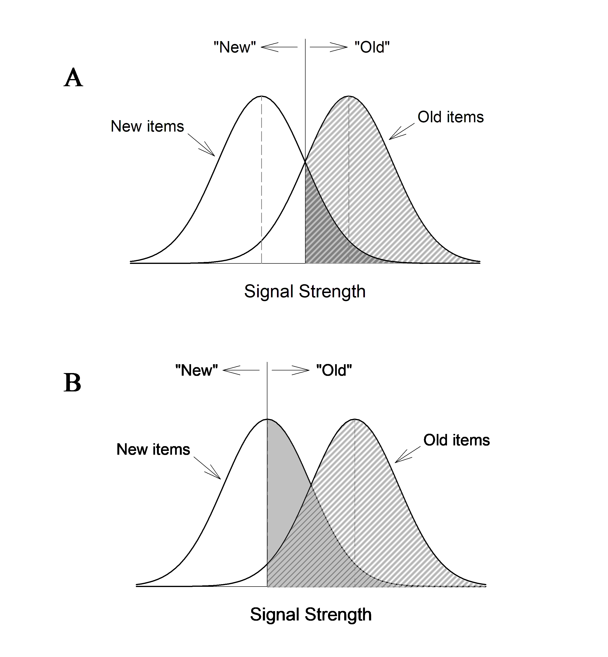
(A) Signal detection interpretation of a participant with an HR of .84 and a FAR of .16 (Participant A). The lighter shaded region corresponds to the HR, and the darker shaded region corresponds to the FAR. (B) Signal detection interpretation of a participant with an HR of .98 and a FAR of .50 (Participant B).
In Figure 2A, the old-item distribution is placed such that 84% of the old items generate a memory signal strong enough to exceed the decision criterion. This is the signal detection interpretation of the participant’s .84 HR. In addition, the new-item distribution is placed such that 16% of the new items also generate a memory signal strong enough to exceed the decision criterion. This is the signal detection interpretation of the participant’s .16 FAR. For two Gaussian distributions that have the same standard deviation (the simplest version of SDT), there is no other way to draw the figure so that it corresponds to Participant A’s pattern of results. It is, therefore, the signal detection interpretation of what is theoretically happening in the unobservable memory of the participant.
The distributions in Figure 2A are two standard deviation units apart. This is theoretically how well Participant A’s brain separates the memory signals of old items and new items. In terms of performance, Participant A is characterized as having achieved a
To see the problem with the use of percent correct from the perspective of SDT, consider the hypothetical performance of Participant B:
Table 4
Basic Performance Measures for Hypothetical Participant B, Who Exhibits a Liberal Response Bias
| “Old” | “New” |
Old | .98 | .02 |
New | .50 | .50 |
Unlike Participant A, whose performance across old and new items was balanced (84% correct for both), Participant B has a response bias to say “old” whenever the item is old or new. This is why almost all of the old items are correctly called “old” (98% correct), but half the new items are incorrectly called “old” as well (50% correct). As before, a natural approach is to average the two “proportion correct” scores:
Figure 2B illustrates the performance of Participant B in terms of SDT. That is, it depicts the signal detection interpretation of the participant’s .98 HR and .50 FAR. Once again, for two Gaussian distributions that have the same standard deviation (i.e., equal variance), there is no other way to draw the figure such that it corresponds to Participant B’s pattern of results. Note that the decision criterion no longer falls midway between the two distributions but is instead shifted to the left. This leftward shift reflects a liberal response bias—that is, the criterion is placed such that Participant B does not require that a test item generate a very strong memory signal to declare it “old.”
Note that the distributions in Figure 2B are also two standard deviation units apart, just as in Figure 2A. In other words, like Participant A, Participant B achieved a
There are various ways to quantify response bias, but a common way is to compute how far the decision criterion is placed from the unbiased placement midway between the two distributions. This measure is usually represented as follows: Participant A has a response bias of
Critically, each participant’s performance is characterized by two measures; one measure reflects the participant’s ability to distinguish between old and new items based on their observable memory signals (
Computing
The computational formula for
Table 5
Data From Five Hypothetical Participants
Participant | HR | FAR | d' | c |
1 | 0.64 | 0.21 | 1.2 | 0.22 |
2 | 0.93 | 0.09 | 2.8 | -0.07 |
3 | 0.48 | 0.00 | undefined | undefined |
4 | 1.00 | 0.40 | undefined | undefined |
5 | 0.72 | 0.18 | 1.5 | 0.17 |
Note. Signal detection metrics cannot be computed for Participant 3 (FAR = 0) or Participant 4 (HR = 1.0).
The
That said, a few participants are likely to have extreme HRs or FARs even after steps have been taken to improve the procedure. The best approach for dealing with those cases is to use a standard correction formula. The idea behind these formulas is that the HR is not truly 1.0, for example, but more trials would be needed to discover its true value. For example, assume that a researcher tests 25 old items, and the participant got all 25 correct (HR = 1.0). Although the HR is probably less than 1.0 (e.g., at least one error would likely occur if many more old items were tested), it is probably greater than
Table 6
Data From Five Hypothetical Participants
Participant | HR | FAR | d' | c |
1 | 0.64 | 0.21 | 1.2 | 0.22 |
2 | 0.93 | 0.09 | 2.8 | -0.07 |
3 | 0.48 | 0.02 | 2.0 | 1.06 |
4 | 0.98 | 0.40 | 2.3 | -0.90 |
5 | 0.72 | 0.18 | 1.5 | 0.17 |
Note. Included in this table are an adjusted FAR for Participant 3 and an adjusted HR for Participant 4.
This allows the computation of the mean value of all four of these measures (HR, FAR,
Questions, controversies, and new developments
SDT has often been the focus of debate, in part because scientists often propose theories in which the underlying signals (e.g., memory signals) are in fact binary, not continuous. These theories often include provisions for randomly guessing “yes” on trials in which a memory signal (or other signal) failed to occur. One challenge for threshold theories is that confidence judgments are naturally graded; participants can report not only whether evidence exceeds a decision threshold but also how strongly the evidence supports their decision. On some trials, the participant will say, “I am 100% sure that this face was on the list.” On other trials, the participant might be 90% confident, or 80% confident, and so on. SDT offers a natural interpretation of these confidence ratings, which simply reflect the continuous nature of the strength of the underlying signal itself (Figure 3).
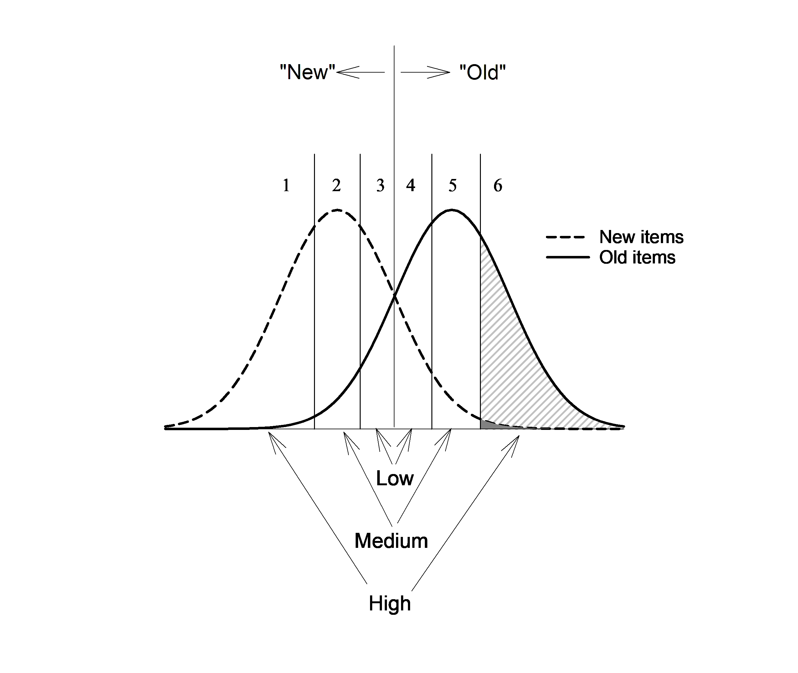
The signal detection interpretation of confidence ratings obtained using a 6-point scale, in which 1 = “definitely new,” 2 = “probably new,” 3 = “maybe new,” 4 = “maybe old,” 5 = “probably old,” and 6 = “definitely old.” The shaded regions to the right illustrate why SDT predicts that decisions made with high confidence will typically be associated with high accuracy (i.e., quite a few old items will be correctly called “old,” but only a few new items will be).
Many debates about SDT surround a method of analysis based on a plot known as the receiver operating characteristic (ROC). As indicated in Figure 2A (neutral response bias) and Figure 2B (liberal response bias), HRs and FARs change as response bias changes, even though
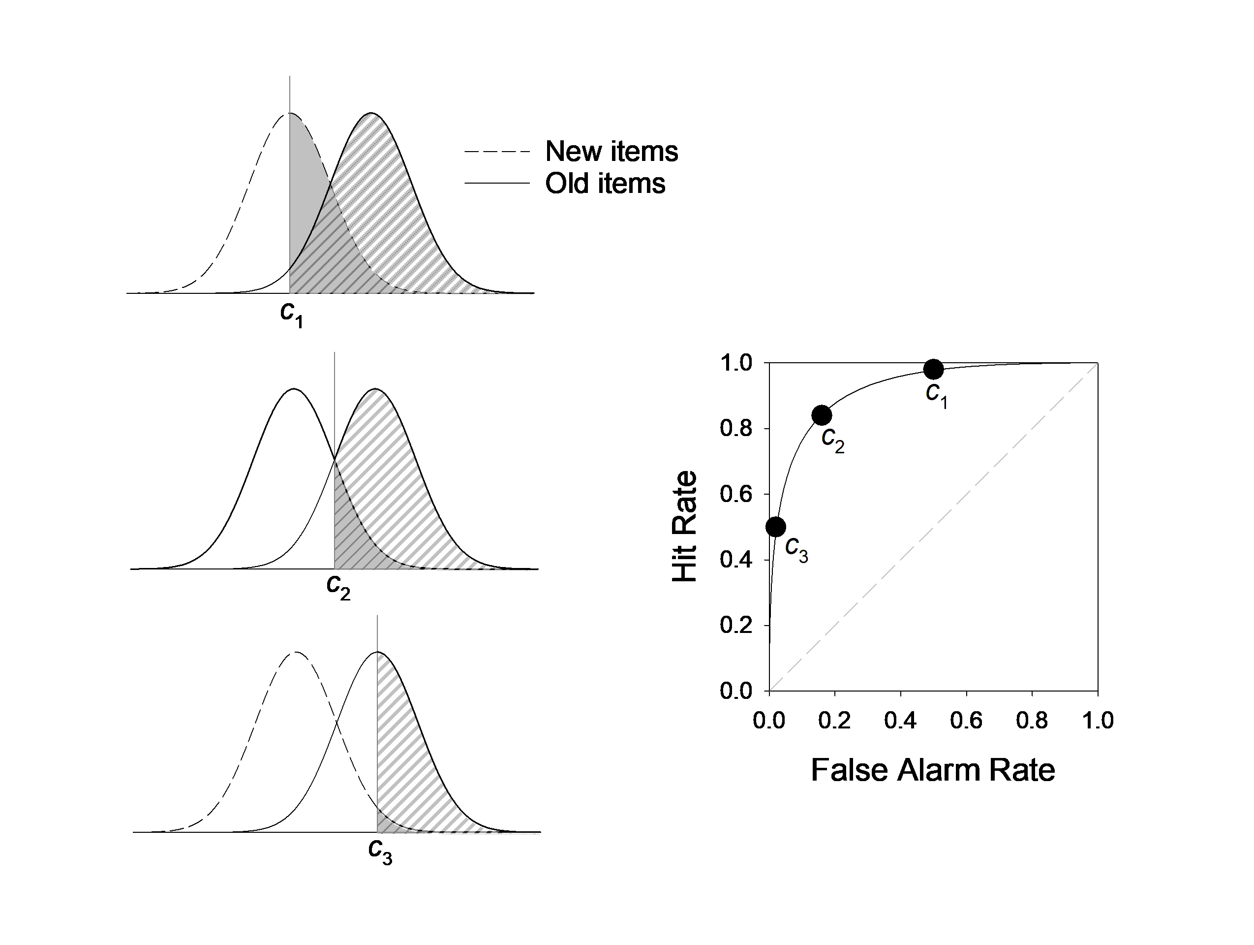
The signal detection interpretation of an ROC plot in which d’ is constant (at 2.0) while the decision criterion changes from liberal (c1) to neutral (c2) to conservative (c3). As with computations of d’ and c, an ROC plot can be constructed separately for each participant based on their confidence ratings or at the group level by pooling confidence ratings across participants.
If a researcher’s goal is to simply measure performance without worrying too much about a quantitative theory, an easy way to avoid contentious measurement issues is to simply use the two-alternative forced-choice task (Fechner, 1860/1966; Thurstone, 1927). In a two-alternative forced-choice task, there is no decision criterion to worry about because on every trial the participant simply selects the item that generates the stronger signal. In that case, even percent correct is a fine measure because, for main effects (condition A vs. condition B), it will always directionally agree with
Broader connections
The modern version of SDT emerged essentially simultaneously from the fields of statistics and psychophysics, which converged in the early 1950s with the realization that ROC analysis offers a powerful way to measure discriminability. The measure is “area under the ROC” curve. The larger that area, the better discriminability is. For applied purposes, in which theoretical assumptions are less central, it is often a more robust measure than
Beyond its role as a measurement tool, however, SDT provides a general framework for modeling decision-making under uncertainty. In this framework, behavior reflects the joint influence of underlying evidence strength and decision criteria, allowing theoretically meaningful dissociations between sensitivity (e.g.,
These theoretical commitments extend naturally to neuroscience. Neural activity in sensory and associative cortices is often interpreted as reflecting the momentary strength of evidence, linking neural discriminability to behavioral sensitivity (Britten et al., 1992). Decision-related activity in frontal and parietal regions has likewise been linked to the accumulation of evidence toward a response and to criterion-like decision processes (Gold & Shadlen, 2007; Shadlen & Newsome, 2001). Trial-by-trial variability in neural firing can account for psychophysical sensitivity, providing a bridge between SDT measures such as
In the 1970s and 1980s, and continuing to this day, the field of diagnostic medicine adopted ROC analysis as the gold standard for assessing the efficacy of diagnostic tests (e.g., Metz, 1978). This is an example of a domain in which the emphasis is on decision performance—such as how well a test discriminates individuals with and without a disease—rather than on specifying the underlying generative model. Today, the same framework underlies analyses in psychology, neuroscience, engineering, and machine learning (Swets et al., 2000), particularly for evaluating classification performance and threshold trade-offs [see AI Model Evaluation]. In modern machine learning, ROC curves and area under the curve are standard tools for assessing classifier performance across decision thresholds, reflecting the same sensitivity bias trade-off formalized by SDT. Applied domains such as eyewitness identification similarly rely on ROC analysis to assess discriminability independent of response bias (Mickes et al., 2012).
Finally, ongoing extensions of SDT, including unequal-variance models, hierarchical formulations, and models that incorporate confidence and response time, underscore its continued development as a flexible framework for linking observable behavior to underlying cognitive and neural processes.
Further reading
Hautus, M. J., Macmillan, N. A., & Creelman, C. D. (2022). Detection theory: A user’s guide (3rd ed.). Routledge.
Green, D. M., & Swets, J. A. (1966). Signal detection theory and psychophysics. Wiley.
Wixted, J. T. (2020). The forgotten history of signal detection theory. Journal of Experimental Psychology: Learning, Memory, and Cognition, 46(2), 201–233. https://doi.org/10.1037/xlm0000732
References
Blackwell, H. R. (1953). Psychophysical thresholds: Experimental studies of methods of measurement. University of Michigan Press.
↩Brady, T. F., Robinson, M. M., Williams, J. R., & Wixted, J. T. (2023). Measuring memory is harder than you think: How to avoid problematic measurement practices in memory research. Psychonomic Bulletin & Review, 30(2), 421–449. https://doi.org/10.3758/s13423-022-02179-w
↩Britten, K. H., Shadlen, M. N., Newsome, W. T., & Movshon, J. A. (1992). The analysis of visual motion: A comparison of neuronal and psychophysical performance. The Journal of Neuroscience, 12(12), 4745–4765. https://doi.org/10.1523/JNEUROSCI.12-12-04745.1992
↩Fechner, G. T. (1966). Elements of psychophysics (H. E. Adler, Trans.). Holt, Rinehart & Winston. (Original work published 1860)
↩Gold, J. I., & Shadlen, M. N. (2007). The neural basis of decision making. Annual Review of Neuroscience, 30, 535–574. https://doi.org/10.1146/annurev.neuro.29.051605.113038
↩Hautus, M. J., Macmillan, N. A., & Creelman, C. D. (2022). Detection theory: A user’s guide (3rd ed.). Routledge.
↩Link, S. W. (1994). Rediscovering the past: Gustav Fechner and signal detection theory. Psychological Science, 5(6), 335–340. https://doi.org/10.1111/j.1467-9280.1994.tb00282.x
↩Metz, C. E. (1978). Basic principles of ROC analysis. Seminars in Nuclear Medicine, 8(4), 283–298. https://doi.org/10.1016/S0001-2998(78)80014-2
↩Mickes, L., Flowe, H. D., & Wixted, J. T. (2012). Receiver operating characteristic analysis of eyewitness memory: Comparing the diagnostic accuracy of simultaneous versus sequential lineups. Journal of Experimental Psychology: Applied, 18(4), 361–376. https://doi.org/10.1037/a0030609
↩Shadlen, M. N., & Newsome, W. T. (2001). Neural basis of a perceptual decision in the parietal cortex (area LIP) of the rhesus monkey. Journal of Neurophysiology, 86(4), 1916–1936. https://doi.org/10.1152/jn.2001.86.4.1916
↩Swets, J. A. (1961). Is there a sensory threshold? Science, 134(3473), 168–177. https://doi.org/10.1126/science.134.3473.168
↩Swets, J. A. (1986). Indices of discrimination or diagnostic accuracy: Their ROCs and implied models. Psychological Bulletin, 99(1), 100–117. http://doi.org/10.1037/0033-2909.99.1.100
↩Swets, J. A., Dawes, R. M., & Monahan, J. (2000). Psychological science can improve diagnostic decisions. Psychological Science in the Public Interest, 1(1), 1–26. http://doi.org/10.1111/1529-1006.001
↩Tanner, W. P., Jr., & Swets, J. A. (1954). A decision-making theory of visual detection. Psychological Review, 61(6), 401–409. http://doi.org/10.1037/h0058700
↩Thurstone, L. L. (1927). A law of comparative judgment. Psychological Review, 34(4), 273–286. https://doi.org/10.1037/h0070288
↩Yonelinas, A. P. (1994). Receiver-operating characteristics in recognition memory: Evidence for a dual-process model. Journal of Experimental Psychology: Learning, Memory, and Cognition, 20(6), 1341–1354. https://doi.org/10.1037/0278-7393.20.6.1341
↩