The drift diffusion model (DDM) is an account of how binary decisions are made based on noisy pieces of information. Noisy information is translated into evidence favoring one option or the other and accumulated until there is sufficient net evidence favoring an option, akin to a tug-of-war. The DDM explains both the degree of choice consistency/accuracy and the time that it takes to make decisions. In cases in which one option is clearly favored over the other, evidence consistently points in the same direction, and the resulting choices are quick and consistent. In cases in which the options are similarly supported, choices are slow and inconsistent. The DDM explains the speed–accuracy trade-off because demanding more net evidence leads to more accurate/consistent decisions but also requires more time. The DDM has several important properties. Under reasonable assumptions, it is an optimal decision-making procedure—for a desired accuracy, it minimizes the average reaction time (RT). It provides an accurate account of choice and RT data across a wide variety of domains, including perception, memory, and preference. Finally, it is supported by neuroscience research showing that choice-related neural activity rises noisily until a constant threshold is reached, prompting a choice.
History
The DDM, also known as the diffusion decision model, is the canonical sequential sampling model, also sometimes called evidence-accumulation or accumulation-to-bound models. These models originate in statistics, from which Abraham Wald (1945) introduced the sequential probability ratio test, an optimally efficient procedure for deciding between two hypotheses based on randomly distributed (i.e., noisy) data. Cognitive scientists later applied Wald’s model to human choice and RT data. At the time, a perceived problem with the DDM was that it predicted identical RT distributions for correct and error choices, but this was rarely observed in reality. Roger Ratcliff (1978) solved this problem by introducing across-trial variability in the evidence-accumulation (drift) rates. By doing so, Ratcliff allowed the DDM to account for the typical pattern of slow errors and opened the door for cognitive psychologists to use the DDM as both a model of cognition and an analysis tool.
Meanwhile, in neuroscience, researchers identified neural signatures of a DDM-like process (Hanes & Schall, 1996; Shadlen & Newsome, 2001). Notably, Michael Shadlen recorded activity from neurons responsible for response execution (i.e., eye movements) while the decision-makers (monkeys) watched flickering dots on the computer screen, trying to discern which way some of the dots were moving (left or right). The data from these experiments showed that activity in the eye movement neurons (in the lateral intraparietal area) rose at a rate proportional to the fraction of moving dots but also reached a constant threshold level of activity immediately before the decision. These features of the neural data align closely with what one would expect from a DDM, that is, noisy accumulation up to a threshold. As a result, the use of the DDM (and related models) in neuroscience has proliferated (O'Connell et al., 2018).
Finally, in the domain of preference-based (i.e., value-based or economic) decisions, the DDM and related models have also taken hold. Decision scientists have expanded on the DDM, starting with decision field theory (Busemeyer & Townsend, 1993) and later incorporating eye movements (Krajbich et al., 2010), attribute latencies (Maier et al., 2020; Sullivan & Huettel, 2021), and neural data (Hare et al., 2011; Gluth et al., 2012; Pisauro et al., 2017) [see Eye Movements; Neuroeconomics].
Core concepts
The DDM is a mathematical model of binary choice that assumes that decision-makers gather evidence over time, keeping a running total of the difference in evidence between the two options and stopping when that total exceeds a predefined threshold (Figure 1). The DDM takes several psychological parameters and produces choice and RT distributions that align with typical empirical patterns, namely logistic choice curves and fat-tailed RT distributions. In other words, the DDM explains the fact that choices are typically more accurate/consistent when one option is more clearly supported over the other and that RTs cannot be negative but can occasionally be quite long. The DDM also predicts longer RTs as choice probabilities approach 50%.
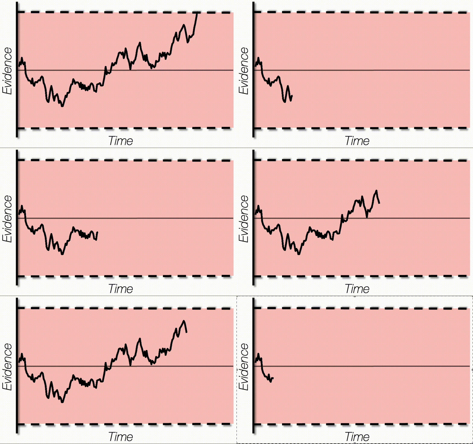
Evolution of a DDM in real time.
The DDM decomposes decision-making into a few key components that are captured with numerical parameters (Figure 2). By adjusting the parameters to best fit the model to data, researchers can examine how these components differ across groups, conditions, and more. The components are as follows:
The drift rate reflects the average incoming evidence supporting one option over the other. Larger drift rates reflect stronger evidence. A drift rate of zero indicates no net support for either option (i.e., indifference). The drift rate can be a simple function of a single dimension of the stimulus or a complex function of multiple of its attributes, possibly with weights that change over time because of shifting attention or considerations. The drift rate captures the difficulty of the decision to the decision-maker and so reflects both the decision-maker’s ability and the inherent discriminability of the options.
The boundary separation is the amount of evidence required to make a decision. The boundary separation controls the speed–accuracy trade-off, with wider boundaries leading to slower but more accurate decisions. We typically assume that the decision-maker sets the boundary separation beforehand.
The diffusion noise is the variability in the incoming evidence from one instant to the next. Each piece of evidence is drawn from a normal distribution with mean equal to the drift rate and standard deviation equal to the diffusion noise. One can think of the ratio of drift rate to diffusion as the signal-to-noise ratio of the choice process.
The starting point of the decision process reflects whether the decision-maker is initially neutral between the two options or has some prior information leading them to initially favor an option. Starting points are often used to capture response bias—the tendency to repeat past actions.
Nondecision time is time that contributes to the decision-maker’s RT but does not involve an evaluation of the options. This nondecision time is meant to capture initial orienting to the options as well as motor latencies involved in making a selection after a decision boundary has been reached.
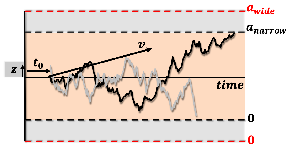
Depiction of the DDM. Shown are two examples of the DDM process, one in black, and one in gray. The decision variable, or net evidence, evolves over time from left to right in the figure until it hits a decision boundary (horizontal dashed lines). The variable v denotes the drift rate for the example in black. The variable z denotes the starting point bias for the example in gray. The variable t0 denotes the nondecision time for both examples. The variable a denotes the boundary separation with the narrow black boundaries used in these examples and the red wide boundaries corresponding to a slower but more accurate decision rule.
When estimating DDM parameters, we must set drift rate, boundary separation, or diffusion noise to a constant. This is because the unit of evidence is arbitrary, meaning that we can scale up the diffusion noise, drift rate, and boundary separation by a constant without changing the model. In most cases, researchers set the diffusion noise to a constant and estimate drift rate and boundary separation.
Across-trial variability in the above parameters is used to account for the fact that these decision components are not identical from one choice to the next. Allowing these parameters to vary is important to account for various patterns in behavioral data such as slow and fast errors.
Questions, controversies, and new developments
The DDM is a model of choices between two options. How the model extends to choices with multiple options is less well understood. With multiple options, there is an asymptotically optimal model (i.e., optimal as accuracy approaches 100%) that compares the option with the most evidence to the option with the next most evidence (Dragalin et al., 1999). However, there is limited research on the multialternative case (Churchland et al., 2008). With a continuum of options, for example, submitting a rating from 0 to 100, there are circular diffusion models that allow evidence to accumulate in two dimensions towards a circular arc, from which the crossing point on the arc determines the response (Smith, 2016).
How might the brain produce DDM-like behavior? There has been debate about whether evidence is accumulated within individual neurons or in the aggregate activity of many neurons in attractor networks (Wong & Wang, 2006; Zoltowski et al., 2019). There is also debate about whether, over time, decision boundaries collapse, urgency signals amplify evidence (Cisek et al., 2009; Hawkins et al., 2015), or evidence leaks out (Usher & McClelland, 2001).
Broader connections
The DDM has connections to statistics. Both the sequential probability ratio test (mentioned above) and Bayesian updating are special cases of the DDM in which what is being accumulated are the log likelihood ratios for each piece of information supporting one option over the other. From the Bayesian perspective, the starting point is the decision-maker’s prior, and the accumulated evidence is their posterior.
Models like the DDM are prevalent throughout the sciences, with the use of Brownian motion and Wiener processes in physics, finance, evolutionary biology, cosmology, and many other subjects. A more general form of the DDM, the Ornstein–Uhlenbeck model, allows for nonlinearities in the diffusion process and is also widely used.
The DDM provides a counterpoint to models of choice selection in which people are thought to use algorithmic or heuristic processes to tackle complex decision problems. It also provides a counterpoint to traditional economic models of rational decision-making that assume stable, known preferences.
Acknowledgments
The author would like to acknowledge National Science Foundation award 2333979 and Kianté Fernandez for research assistance.
Further reading
Bogacz, R., Brown, E., Moehlis, J., Holmes, P., & Cohen, J. D. (2006). The physics of optimal decision making: A formal analysis of models of performance in two-alternative forced-choice tasks. Psychological Review, 113(4), 700-765. https://doi.org/10.1037/0033-295X.113.4.700
Busemeyer, J. R., Gluth, S., Rieskamp, J., & Turner, B. M. (2019). Cognitive and neural bases of multi-attribute, multi-alternative, value-based decisions. Trends in Cognitive Sciences, 23(3), 251-263. https://doi.org/10.1016/j.tics.2018.12.003
Gold, J. I., & Shadlen, M. N. (2007). The neural basis of decision making. Annual Review of Neuroscience, 30(1), 535-574. https://doi.org/10.1146/annurev.neuro.29.051605.113038
Krajbich, I., Fernandez, K., & Yang, X. (2025). Decomposing economic choices with drift-diffusion models. In D. V. Smith, P. L. Lockwood, & D. S. Fareri (Eds.), Neuroeconomics: Core topics and current directions (pp. 141-165). Springer.
Ratcliff, R., & McKoon, G. (2008). The diffusion decision model: Theory and data for two-choice decision tasks. Neural Computation, 20(4), 873-922. https://doi.org/10.1162/neco.2008.12-06-420
References
Busemeyer, J. R., & Townsend, J. T. (1993). Decision field theory: A dynamic-cognitive approach to decision making in an uncertain environment. Psychological Review, 100(3), 432-459. https://doi.org/10.1037/0033-295x.100.3.432
↩Churchland, A. K., Kiani, R., & Shadlen, M. N. (2008). Decision-making with multiple alternatives. Nature Neuroscience, 11(6), 693-702. https://doi.org/10.1038/nn.2123
↩Cisek, P., Puskas, G. A., & El-Murr, S. (2009). Decisions in changing conditions: The urgency-gating model. Journal of Neuroscience, 29(37), 11560-11571. https://doi.org/10.1523/JNEUROSCI.1844-09.2009
↩Dragalin, V. P., Tartakovsky, A. G., & Veeravalli, V. V. (1999). Multihypothesis sequential probability ratio tests-Part I: Asymptotic optimality. IEEE Transactions on Information Theory, 45(7), 2448-2461.
↩Gluth, S., Rieskamp, J., & Büchel, C. (2012). Deciding when to decide: time-variant sequential sampling models explain the emergence of value-based decisions in the human brain. Journal of Neuroscience, 32(31), 10686-10698. https://doi.org/10.1523/JNEUROSCI.0727-12.2012
↩Hanes, D. P., & Schall, J. D. (1996). Neural control of voluntary movement initiation. Science, 274(5286), 427-430. https://doi.org/10.1126/science.274.5286.427
↩Hare, T. A., Schultz, W., Camerer, C. F., O'Doherty, J. P., & Rangel, A. (2011). Transformation of stimulus value signals into motor commands during simple choice. Proceedings of the National Academy of Sciences, 108(44), 18120-18125. https://doi.org/10.1073/pnas.1109322108
↩Hawkins, G. E., Forstmann, B. U., Wagenmakers, E. J., Ratcliff, R., & Brown, S. D. (2015). Revisiting the evidence for collapsing boundaries and urgency signals in perceptual decision-making. Journal of Neuroscience, 35(6), 2476-2484. https://doi.org/10.1523/JNEUROSCI.2410-14.2015
↩Krajbich, I., Armel, C., & Rangel, A. (2010). Visual fixations and the computation and comparison of value in simple choice. Nature Neuroscience, 13(10), 1292-1298. https://doi.org/10.1038/nn.2635
↩Maier, S. U., Raja Beharelle, A., Polanía, R., Ruff, C. C., & Hare, T. A. (2020). Dissociable mechanisms govern when and how strongly reward attributes affect decisions. Nature Human Behaviour, 4(9), 949-963. https://doi.org/10.1038/s41562-020-0893-y
↩O’Connell, R. G., Shadlen, M. N., Wong-Lin, K., & Kelly, S. P. (2018). Bridging neural and computational viewpoints on perceptual decision-making. Trends in Neurosciences, 41(11), 838-852. https://doi.org/10.1016/j.tins.2018.06.005
↩Pisauro, M. A., Fouragnan, E., Retzler, C., & Philiastides, M. G. (2017). Neural correlates of evidence accumulation during value-based decisions revealed via simultaneous EEG-fMRI. Nature Communications, 8(1), 15808. https://doi.org/10.1038/ncomms15808
↩Ratcliff, R. (1978). A theory of memory retrieval. Psychological Review, 85(2), 59-108. https://doi.org/10.1037/0033-295X.85.2.59
↩Shadlen, M. N., & Newsome, W. T. (2001). Neural basis of a perceptual decision in the parietal cortex (area LIP) of the rhesus monkey. Journal of Neurophysiology, 86(4), 1916-1936. https://doi.org/10.1152/jn.2001.86.4.1916
↩Smith, P. L. (2016). Diffusion theory of decision making in continuous report. Psychological Review, 123(4), 425-451. https://doi.org/10.1037/rev0000023
↩Sullivan, N. J., & Huettel, S. A. (2021). Healthful choices depend on the latency and rate of information accumulation. Nature Human Behaviour, 5(12), 1698-1706. https://doi.org/10.1038/s41562-021-01154-0
↩Usher, M., & McClelland, J. L. (2001). The time course of perceptual choice: The leaky, competing accumulator model. Psychological Review, 108(3), 550-592. https://doi.org/10.1037/0033-295x.108.3.550
↩Wald, A. (1945). Sequential tests of statistical hypotheses. The Annals of Mathematical Statistics, 16(2), 117-186. https://doi.org/10.1214/aoms/1177731118
↩Wong, K. F., & Wang, X. J. (2006). A recurrent network mechanism of time integration in perceptual decisions. Journal of Neuroscience, 26(4), 1314-1328. https://doi.org/10.1523/JNEUROSCI.3733-05.2006
↩Zoltowski, D. M., Latimer, K. W., Yates, J. L., Huk, A. C., & Pillow, J. W. (2019). Discrete stepping and nonlinear ramping dynamics underlie spiking responses of LIP neurons during decision-making. Neuron, 102(6), 1249-1258. https://doi.org/10.1016/j.neuron.2019.04.031
↩